Star news


How to find the voltage measurement error. Typical tasks. Resistance measurement errors
Task No. 1………………………………………………………………………………3
Task No. 2………………………………………………………………………………6
Task No. 3………………………………………………………………………………..9
LIST OF SOURCES USED………………………13
Task No. 1. Verification of technical instruments and fundamentals of metrology
Technical ammeter of magnetoelectric system with rated current I nom =5A, number of nominal divisions A nom = 100 has digitized divisions from zero to the nominal value, placed on every fifth of the scale (the arrows of de-energized ammeters occupy the zero position). Absolute error: +0.03, +0.06, -0.05, +0.04, -0.02.
Resistance measurement errors
Error is defined as the difference between the measured or estimated value for a quantity and its true value and is inherent in all measurements. Knowing the type and extent of error that may be present has important, if the data is to be used wisely, regardless of whether the data was considered personally measured or simply read from the manufacturer's data sheets for the material or component. In medical research, biology, and social sciences, the design of data collection and analysis is the basis of the experiment.
The technical ammeter was verified using a standard ammeter of the same system.
1. Specify the conditions for verification of technical devices.
2. Determine measurement corrections.
3. Construct a graph of amendments.
4. Determine the relative error.
5. Determine the reduced error.
6. Indicate which standard accuracy class this device belongs to.
Engineers must also be careful, although some engineering measurements have been made with fantastic precision, most have less than 1 percent error and some must use advanced experimental design and analysis techniques to obtain any useful data. Taking measurements and analyzing them is a key part of the design process, from the initial characterization of materials and components needed for design, to prototype testing, quality control during production, operation and maintenance final product.
If the device does not comply with the established accuracy class, please indicate this specifically.
1. Verification is carried out in a room with normal conditions for working devices. The ammeter is checked by comparing the readings of a standard ammeter. In an ammeter with accuracy class 1.0; 1.5; 2.5; 5.0 is checked by comparing their readings with the readings of samples of devices of class 0.2 and 0.5.
Additionally, you need to include the reasoning and calculations that went into your error estimate if it is to be believable to others. The advantage of the fractional error format is that it gives an idea of the relative importance of the error.
Errors can be divided into roughly two categories: Systematic error in a measurement is a consistent and repeatable bias or offset from the true value. This is usually the result of a miscalculation of the test equipment or problems with the experimental procedure. On the other hand, variations between successive measurements made under apparently identical experimental conditions are called random errors. Random variations can occur either in the measured physical quantity or in the measurement process, or in both cases.
2. Knowing the absolute error for each digitized scale division (1; 2; 3; 4; 5). We determine the measurement corrections, taking into account that the correction is the absolute error taken with the opposite sign:
- θ 1 = -0,03
- θ 2 = -0,06
- θ 3 = +0,05
- θ 4 = -0,04
- θ 5 = +0,02
3. To construct a graph of corrections, we draw coordinate axes: horizontal, on which the digitized values of the scale divisions will be plotted, and vertical - to plot corrections - up positive, down negative.
We describe statistical procedures to handle this type of error. When presenting experimental results, a distinction should be made between "precision" and "precision". Accuracy is a measure of how closely a measured value matches the true value. A very accurate measurement has very little error associated with it. Note that in experimental work the true value is often unknown and therefore the information reported must be the estimated precision or error.
Resistance measurement methods
Accuracy is a measure of the repeatability and resolution of a measurement—the smallest change in the quantity being measured that can be detected reliably. High precision experimental equipment can consistently measure very small differences in a physical quantity. Please note that a highly accurate measurement may still be quite inaccurate. High measurement accuracy is a necessary but not sufficient condition for high accuracy.
4. The relative error is calculated using the formula:
![]()
where X and is the measured value of the quantity;
X d is the actual value of the quantity.
5. Based on the definition given above, the given error is determined by the formula:
![]() ,
,
Suppose that when measuring the voltage, the engineer gets an average reading of 1 volt and that the rightmost digit flickers up and down between 0, 1 and 2, seemingly randomly. Thus, the accuracy in absolute terms is approximately volts. Accuracy can be assessed from the measurements obtained; accuracy must be found in comparison with an accepted voltage standard. By looking at the manufacturer's specification sheet, which includes the results of this comparison, the engineer considers the voltmeter's rated accuracy.
The Seebeck coefficient is one of the key quantities of thermoelectric materials and is regularly measured in various laboratories. However, there are several ways to calculate the Seebeck coefficient from raw measurement data. We compare these various ways extracting the Seebeck coefficient, assessing the accuracy of the results, and showing methods for improving this accuracy. In addition, we indicate experimental and data analysis parameters that can be used to evaluate the validity of the obtained result.
where X n and X k are the starting and ending points of the instrument scale;
X and is the measured value of the quantity;
X d is the actual value of the quantity;
D – measurement range.
The remaining calculation results were performed similarly and are included in Table 1.
Table 1
6. The accuracy class of a measuring instrument is a generalized characteristic determined by the limits of permissible basic and additional errors, as well as other properties affecting accuracy, the values of which are established in the standards for certain types of measuring instruments.
The presented analysis can be used to find and minimize measurement errors of the Seebeck coefficient and, therefore, increase the reliability of the measured material properties. Thermoelectric materials can convert heat directly into useful electrical energy. Since there are ubiquitous sources of heat transfer, readily available thermoelectric generators have many potential applications; they can, for example, improve the fuel efficiency of cars or power sensors.
The attractiveness of thermoelectric generators is related to their efficiency in converting electrical energy. Many systematic errors in Seebeck coefficient measurements are due to hardware problems such as thermal contact resistance between the sample and the thermocouple, stray heat flow through the thermocouples, and other sources. In this article, we will focus on appropriate data analysis for the Seebeck coefficient, highlighting the consistency checks that can be made to assess the validity of the data obtained, and identifying parameters that highlight measurement problems.
The largest reduced error of the device in percentage at all marks of the working part is equal in absolute value to 1.2%, so we determine the accuracy class (the closest normalized value exceeding the value of the reduced error) from the standard series. The accuracy class of the ammeter being verified is 1.5.
Task No. 2. Methods and errors of electrical measurements
We will present the setup used shortly. It shares many features with other installations and can therefore serve as a typical example. The focus here is not on the actual hardware design details; a brief introduction is nevertheless useful for the following discussion.
The sample is subjected to a variable temperature gradient, which can be created using gradient heaters located near the sample. Drawing. The pattern of the Seebeck coefficient is determined in a sequence of measurements as shown in the figure. After a certain time, usually 60 s, the heater turns off, the temperature gradient relaxes, and the voltage signals slowly disappear. After the system has approximately returned to the equilibrium heater 2, power up and repeat the step.
To measure resistance by indirect method, two instruments were used: an ammeter and a voltmeter of the magnetoelectric system.
Resistance measurements were carried out at a temperature t°C with devices of group 2, 5 or 6. Data of the devices, their readings, as well as the group of devices and the ambient temperature at which the resistance was measured, U nom = 30V, I total = 7.5 mA, = 1.0%, U =18V, I nom =15A, U pad =100mV, =1.5%, I=8A, device group 6, t=40 ºС
Following Martin's classification scheme, the measurement procedure is thus quasi-stationary. To prevent crosstalk between the recorded voltage signals and the power supplied to the gradient heaters, only data obtained after the heaters are turned off is used for subsequent analysis. Since the setup contains only two thermocouples, one multimeter and a switch card, it is one of the simplest systems for measuring the Seebeck coefficient. Therefore, many things discussed below are representative of other systems, even though details in the hardware or electronics may differ.
Define:
1) resistance value r’ x according to instrument readings and draw a diagram;
2) resistance value r x taking into account the device connection diagram;
3) the most possible (relative δ and absolute Δ) errors in the measurement result of this resistance;
4) within what limits are the actual values of the measured resistance.
We now want to estimate several equations that can be used to obtain the Seebeck sampling coefficient. Reorganizing the equations gives the first two equations. This is due to the thermocouple manufacturing process and cannot be avoided. On the other hand, it is desirable that the temperature difference created across the sample during measurement be small, so that simplification in the equation holds. Consequently, in practice the equations tend to give incorrect results and are rarely used as such.
The second reason the equation is questionable is the existence of small spurious voltages from within the measurement system. They may be due to differences in temperature at any electrical connection between different materials or inhomogeneities in thermocouples and usually cannot be completely eliminated.
1. Resistance value R'x determined by the formula:
where U is the voltmeter reading, V;
I – ammeter readings, A.
![]()
To choose the right schema, you must first define the relationships and
where U pad is the voltage drop at the device terminals, mV;
It can be seen that the obtained measurement data can be represented well by the formula using the given parameters. The example illustrates that the equation should only be used to obtain a rough estimate of the Seebeck coefficient of a sample. A well-known approach to eliminating the effect of offsets is to derive the Seebeck coefficient not from a single set of data points, but from a linear fit between voltage and temperature difference. For the equations to be correct, it is only necessary for the offsets to be constant during the measurement, which can be done experimentally much more simply than having no offsets at all.
I nom – measurement limit, A.
![]()
where U nom – measurement limit, V;
I full – current of full deflection of the instrument needle, mA.
![]()
![]()
![]()
The figures show the original measurement data, the corresponding linear values corresponding to the data, and the linear correlation coefficients and Seebeck coefficients that were calculated from the fit. The Seebeck coefficient values obtained from the three linear additives are very similar and differ by less than 1%. Other differences may be caused by statistical noise in the measurement signals and small inaccuracies in the Seebeck coefficient of the wire material.
For each temperature, linear correlation coefficients were calculated for all three data sets. In short, the equations give very similar results for the Seebeck coefficient and are equivalent. This may not be too surprising since they are derived from the same basic equations and describe the same physical situation. However, as will be shown below, the observed good agreement is not self-evident and can easily be violated. For the results shown so far, the temperatures used in the equations are not obtained from the multimeter temperature reading.
Select a scheme:
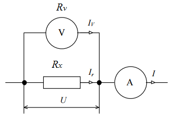
2. Find the resistance value R x taking into account the device connection diagram
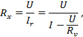
where U – voltmeter readings, V;
I – ammeter readings, A;
R v – internal resistance of the voltmeter, Ohm.
The relationship between the voltage from the thermocouple and the corresponding temperature at the junction is given by the formula. It should also be noted that small errors in temperature measurement have virtually no effect on the result for the Seebeck coefficient if they remain constant. In fact, if we assume the single cold junction temperature for two thermocouples that actually have different cold side junction temperatures, one or both of the calculated temperatures will differ from its "true" value.
If only the temperature readings from the multimeter are used instead, the convention is less effective. Another benefit compared to improved accuracy is external voltage and temperature conversion. This switching takes some time due to internal stabilization procedures and limits the number of measured data points in a transient measurement procedure as used in our setup. If only voltages are recorded, more data points can be obtained in the same measurement time, reducing the statistical uncertainty of the results obtained.
![]()
2. Find the most possible (relative δ and absolute Δ) errors in the measurement result of this resistance:
![]() .
.
1) For voltmeter
±γ v =±1.0±1.0=±2%
2) For ammeter
±γ a =±1.5±1.5=±3%
The relative error in the indirect method of measuring resistance is determined by the formula
![]() ,
,
where δ U and δ I- relative errors in measuring voltage and current.
Values δ U and δ I can be determined using the formulas given in the recommended literature. Thus, the relative error when measuring voltage will be
where γ Σ is the most possible error of the measurement result;
U nom - rated voltage of the voltmeter;
U is the measured voltage value.
![]()
The relative error is determined similarly when measuring current:
![]()
±δ R =±3.33±5.6=±8.93%,
To determine the absolute error, as well as the limits of change in the actual value of the measured resistance R you should use the ratio
![]()
![]()
![]()
4. Real values measured resistance are within:
R x -∆R≤R x ≤R x +∆R,
2.05≤R x ≤2.45
Task 3. Measuring magnetic quantities
Magnetic measurements form an integral part of all electrical measuring equipment. At the same time, the share of magnetic measurements among others is continuously increasing. This is explained by the increasingly widespread use of magnetic phenomena in science and technology, a significant increase in the production of ferromagnetic materials (FMM) and their use in electrical devices, instruments and automation.
The classification of magnetic measurement methods is based on the physical essence of the phenomena used for the measurement process, i.e. conversion of a magnetic quantity into an electrical signal.
In this regard, there are induction methods for measuring magnetic quantities; methods based on the interaction of two magnetic fields; methods based on the influence of a magnetic field on the physical properties of substances.
Methods for measuring magnetic quantities form the basis for testing magnetic materials. All ferromagnetic materials are divided into hard magnetic (HMM) and soft magnetic (MMM). The former are used as sources of constant magnetic fields (PM permanent magnets). To date, three areas of testing have developed for them: research of the properties of MTM, production control of MTM samples, production control of permanent magnets. When studying the properties of MTM, it is necessary to obtain fairly complete information about the properties of the material: the initial magnetization curve, the limiting magnetic hysteresis loop, return curves for various points of the demagnetizing section, etc. Induction measurements are carried out, as a rule, by induction and galvanomagnetic converters. Measuring field strength usually comes down to measuring current in magnetizing devices or obtaining information about the tangential component of the field strength from induction or galvanomagnetic converters. Magnetization reversal of MTM can be carried out by constant and alternating fields. When a material is magnetized by a constant field, static characteristics are obtained. With a continuous cyclic change in the field, dynamic characteristics are obtained, which in the infra-low frequency range of magnetization reversal can be approached to static ones with the required accuracy.
To ensure the correctness of the MTM production process and the corresponding correction of the technological regime, the most important individual parameters of the material are controlled, in particular, the coercive force Hc. The algorithm for obtaining Hc is reduced to fixing zero values of magnetic induction or magnetization and reading the field strength.
The classification criteria for monitoring permanent magnets are based on the type of parameters being monitored and the method of obtaining information. A distinction is made between magnetic flux control in a system close to the working one; control along the demagnetizing section. According to the method of obtaining output information, a distinction is made between devices with direct reading and a differential measurement method - obtaining information in the form of the difference in the characteristics of the reference and tested PM.
Magnetically soft materials are characterized by magnetic parameters measured in constant and alternating fields. The main measured characteristics in constant fields for MMM are: the main magnetization curve, the limiting hysteresis loop and its parameters (Br, Hc), the initial and maximum magnetic permeability. GOST 8.377-80 establishes as the main ballastic method for studying the properties of the material. Currently, due to the development by industry of unified electronic devices The method of a continuous slowly varying field has become widespread.
In alternating fields, the main characteristics of the MMM are the main dynamic magnetization curve, dynamic hysteresis loop, complex magnetic permeability and specific losses. In addition, depending on the frequency range of the test, there are a number of other characteristics and parameters to be determined. The most common tests of MMMs are in the frequency range 50 Hz – 10 kHz. The main testing methods in this frequency range are: induction using an ammeter, voltmeter, wattmeter; induction using phase-sensitive devices (ferrometric); induction using potentiometer alternating current; induction using ferrogaf (oscilloscope); induction using stroboscopic transducers; parametric (bridge).
Induction methods are characterized by measuring EMF induced in measuring coils. The use of an ammeter and a voltmeter makes it possible to determine the dynamic relative permeability. Being the simplest, this measurement method has a large error (up to 10%) and does not provide the ability to determine losses in samples. The use of a wattmeter is standardized for determining losses in MMM samples.
The advantages of the wattmeter method are simplicity and high productivity, a relatively small measurement error for industrial tests (5 - 8%), a wide test frequency range (up to 10 kHz). The disadvantages include a small amount of information and an increase in the error during magnetization reversal to an induction of over 1.2 Tesla due to the deviation of the curve shape from sinusoidal.
The ferrometric measurement method is based on the determination of instantaneous values of periodic non-sinusoidal quantities using phase-sensitive devices. The connection between the average value of the derivative of a function and the instantaneous value of the function itself is the basis for the use of inertial instruments for recording the dynamic characteristics of MMM.
The advantages of the ferrometric measurement method include: small error (2 – 5%); the ability to determine a large number of magnetic characteristics, including calculation of losses. The disadvantages of this method are the limited sample size and frequency range; duration of the measurement process and results processing; relatively high cost of devices.
The oscillographic method is used to measure and visually observe the main dynamic magnetization curve, a family of symmetrical hysteresis loops, and losses in samples at frequencies from 50 to 500 Hz. The disadvantages of this method include the need for measurements on the oscilloscope screen, which is associated with an increase in objective and subjective reading errors.
The most accurate of the induction methods for testing MMMs is potentiometric, based on measuring signals proportional to B and H using alternating current potentiometers. This method determines the dependence of magnetic induction on magnetic field strength, the components of complex magnetic permeability, and total losses. The advantages of the method are high measurement accuracy and a wide range of measured values. The disadvantages include: the duration of the measurement process, the high cost of the equipment used and its complexity.
The essence of the stroboscopic measurement method is that the studied periodically changing signals of arbitrary shape are multiplied by the so-called strobe pulse. In this case, multiplication in each subsequent period occurs with a time shift by a certain interval (reading step) in relation to the previous one. As a result, it is possible to make and then reproduce a point-by-point reading of the entire period of the signal under study. This makes it possible, like the ferrometric method, to use inertial recorders and digital printing devices to record rapidly changing processes. The main advantage of the stroboscopic measurement method is the possibility of obtaining documentary information about the characteristics of FMMs in the process of magnetization reversal of the latter.
The parametric method of testing magnetic materials consists of determining the inductance and resistance of the coil with the magnetic circuit under test by balancing the bridge circuit. This method is mainly intended for determining characteristics in the weak field region. Its advantages are: high measurement accuracy, wide test frequency range. The disadvantages include: dependence of the measurement results on inductive and capacitive interference created by the elements of the measurement circuit; increase in error at low test frequencies; complexity and duration of the testing process. There are other methods for testing MMMs in the dynamic magnetization reversal mode, but the technical and operational characteristics of devices based on them are not effective under mass testing conditions.
1.1. A voltmeter of accuracy class 1.0 with a measurement limit of 300 V, having a maximum number of divisions of 150, was verified at 30, 60, 100, 120 and 150 divisions, and the absolute error at these points was 1.8; 0.7; 2.5; 1.2 and 0.8 V. Determine whether the device corresponds to the specified accuracy class, and the relative errors at each mark.
Solution. A voltmeter of accuracy class 1.0 with a measurement limit of 300 V has the greatest absolute error of 3 V. Since the value of the absolute error at all verified marks is less than 3 V, the device corresponds to accuracy class 1.0.
Relative errors:
1.2. It is necessary to measure the consumer current in the range of 20 - 25 A. There is a microammeter with a measurement limit of 200 μA, an internal resistance of 300 Ohms and a maximum number of divisions of 100. Determine the shunt resistance to expand the measurement limit to 30 A and determine the relative measurement error at 85 divisions, if instrument accuracy class 1.0.
Solution. You must first determine the shunt coefficient: ![]() . Then
. Then ![]() . Let's determine the ammeter reading corresponding to 85 divisions, for which we multiply the division price of 0.3 A/division by the number of divisions 85, then the device will show I = 25.5 A. The relative error at this point is DI max = 0.3A.
. Let's determine the ammeter reading corresponding to 85 divisions, for which we multiply the division price of 0.3 A/division by the number of divisions 85, then the device will show I = 25.5 A. The relative error at this point is DI max = 0.3A.
1.3. An ammeter, voltmeter and wattmeter are connected to the AC network through a current transformer of 100 / 2.5 A and a voltage transformer of 600 / 150 V, which showed 100, 120 and 88 divisions, respectively. The measurement limits of the devices are as follows: ammeter - 3 A, voltmeter - 150 V, wattmeter - current 2.5 A, voltage 150 V. All devices of accuracy class 0.5 have a maximum number of divisions 150. Determine the total power consumed by the network, its total resistance and power factor; the greatest absolute and relative error in measuring impedance, taking into account the accuracy class of the instruments.
Solution. We determine the division price of each device as the ratio of the measurement limit to the maximum number of divisions. For an ammeter, the division price is 0.02 A/div, for a voltmeter - 1 V/div, for a wattmeter - 2.5 W/div.
Then the instrument readings: I = 0.02 × 100 = 2A; U = 1 × 120 = 120 V; P = 2.5 × 88 = 220 W.
Transformation coefficients K I = I 1nom / I 2nom = 100 / 2.5 = 40; K U = U 1nom / U 2nom = 600 / 150 = 4.
Then the current, voltage and active power of the network:
The total power consumed by the network is determined through current and voltage:
Power factor
![]() .
.
Network impedance
![]() Ohm.
Ohm.
Highest value impedance
![]() Om,
Om,
where does the absolute error come from?
Relative measurement error
![]() %.
%.
1.4. Using the ammeter and voltmeter method, resistance is measured according to the diagram in Fig. 8.2, A. The ammeter and voltmeter readings were as follows: U = 4.8V, I = 0.15A. The devices have an accuracy class of 1.0 and measurement limits I pr = 250 mA, U pr = 7.5 V. Determine the measured resistance, the largest absolute and relative measurement errors.
Solution. Measured resistance ![]() Ohm. The greatest absolute error of a voltmeter and ammeter, respectively, with the specified limits and accuracy class of 1.0 V; A. The highest value of the measured resistance, taking into account the accuracy class of the devices used, Ohm. Then the relative measurement error is %.
Ohm. The greatest absolute error of a voltmeter and ammeter, respectively, with the specified limits and accuracy class of 1.0 V; A. The highest value of the measured resistance, taking into account the accuracy class of the devices used, Ohm. Then the relative measurement error is %.
1.5. Passport data of the electric energy meter: 220 V, 10 A, 1 kWh – 640 disk revolutions. Determine the relative error of the meter and the correction factor if it was tested at rated current and voltage values and for 10 minutes. made 236 revolutions.
Solution. We determine the nominal and real constants of the counter:
![]() W×s/rev.
W×s/rev.
Meter correction factor ![]() .
.
Relative meter error %.
1.6. The secondary winding of the TKL-3 current transformer is designed to connect an ammeter with a measurement limit of 5 A. The accuracy class of the devices is 0.5. Determine the rated current in the primary circuit and in the ammeter, the measurement errors of devices, if the transformation ratio K I = 60, and the primary circuit current I 1 = 225 A.
1.7. 100 V voltmeter with 100 division scale connected to secondary winding voltage transformer NOSK-6-66 (U 1 = 6000 V). Determine the network voltage if the voltmeter needle stops at the 95th division. Determine the errors when measuring with first class accuracy instruments.
Solution. Based on the voltage transformer data, we determine the transformation ratio: ![]() . Voltage in the primary circuit when the device is displayed. Relative error of voltmeter voltage measurement
. Voltage in the primary circuit when the device is displayed. Relative error of voltmeter voltage measurement ![]() . General relative error.
. General relative error.
1.8. An ammeter of 5 A, a voltmeter of 100 V and a wattmeter of 5 A and 100 V (with a scale of 500 divisions) are connected through a measuring current transformer TSHL-20 10000/5 and a voltage transformer NTMI-10000/100 for measuring current, voltage and power . Determine the current, voltage, active power and power factor of the primary circuit, if in the secondary circuit of the measuring current transformers I 2 = 3 A, voltage U 2 = 99.7 V, and the wattmeter readings are 245 divisions.
Solution. Rated current transformer ratio ![]() . Rated voltage transformer ratio
. Rated voltage transformer ratio ![]() . Current in the primary winding of a transformer. Circuit voltage. Active power of the circuit. Circuit power factor
. Current in the primary winding of a transformer. Circuit voltage. Active power of the circuit. Circuit power factor ![]() .
.